Single-Shot 3D SIM: How a Spinning Disk Reconstructs an Image
On this page
What if the microscope could reconstruct a super-resolved image before the camera finished its exposure?
That is the idea behind our single-shot 3D structured illumination microscopy (3D SIM): a spinning disk patterns the excitation and demodulates the returning fluorescence, producing one optically reconstructed section per camera exposure.
By Youchang Zhang (Joshua Zhang) · An introduction to our 2023 Biomedical Optics Express paper.
1. From fifteen images to one exposure
Conventional three-beam 3D SIM records five illumination phases at three orientations—15 raw images per axial position—and reconstructs the result computationally. Our spinning-disk implementation performs the modulation and demodulation optically during a single exposure.
The reported instrument combines:
- Approximately twofold resolution improvement laterally and axially.
- Up to 100 optical-section images per second, limited by the camera.
- Approximately 90% rejection of out-of-focus background, explained by the disk's opaque area.
Here, single-shot means one exposure per optical section. A complete 3D volume still requires a depth stack. Fewer raw frames also do not, by themselves, establish a fifteenfold speed increase under matched imaging conditions.
See the original paper and experimental images →
2. One disk, two optical jobs
The disk contains a periodic array of pinholes in an opaque coating. On the outward path, it diffracts the excitation into one central beam and four tilted beams. Their interference creates an illumination lattice that varies across the sample and through depth.
On the return path, the objective images the fluorescence onto the same disk. The pinhole pattern modulates it again. As the disk scans, matched illumination–detection contributions survive the camera's integration, while mismatched terms average away in the ideal uniform scan.
This second modulation is the crucial step: it restores the fine-detail information to its original spatial frequency. Meanwhile, the opaque coating blocks much of the out-of-focus fluorescence. Optical reconstruction and background rejection work together.
3. The mathematics behind the shift
3.1 Shift the detail in, then shift it back
Let describe the object's spatial frequencies, and the ordinary microscope's optical transfer function (OTF). Larger means finer detail. Without SIM, the image spectrum is , so information outside the OTF cutoff is lost.
Consider one illumination order that shifts the object spectrum by . After passing through the microscope, its contribution is proportional to
The matching return modulation shifts the whole expression by :
The object spectrum returns to its original position; the OTF window moves with it. For example, a detail at , beyond the ordinary cutoff , can shift to and then back to . It retains the nonzero transfer weight acquired inside the passband.
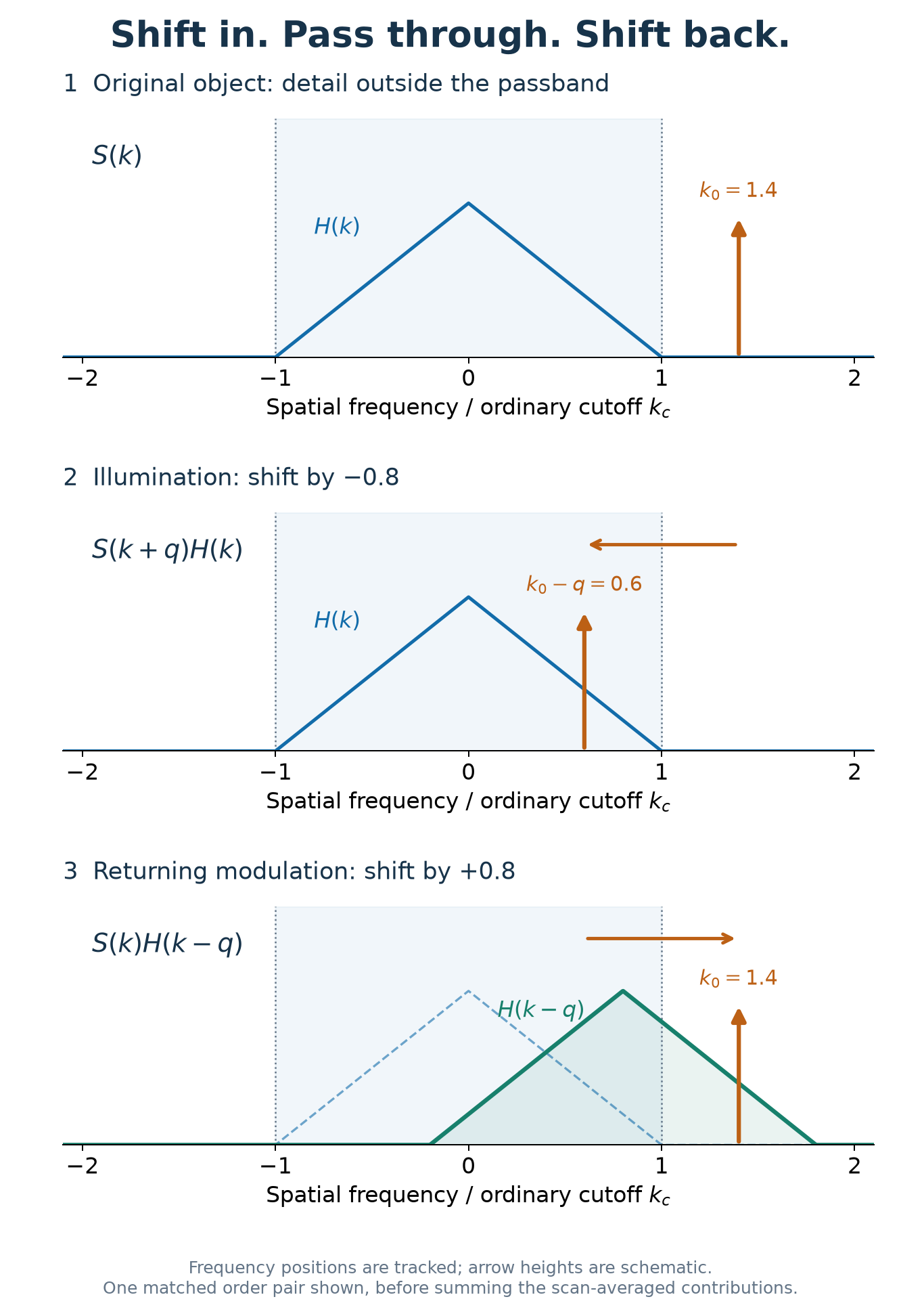 Figure 1. One matched order pair shifts a detail into the ordinary passband and restores it at its original frequency. Frequencies are normalized by the cutoff. The triangular OTF and arrow heights are schematic, not measured amplitudes.
3.2 Restored frequencies, broader OTF
After averaging the matched pairs, their shifted OTF windows add:
Here, labels the pattern frequencies and their weights. Each window keeps its width, but their combined support is wider. The lens itself has not changed; the complete illumination–detection system transfers a broader range of object detail.
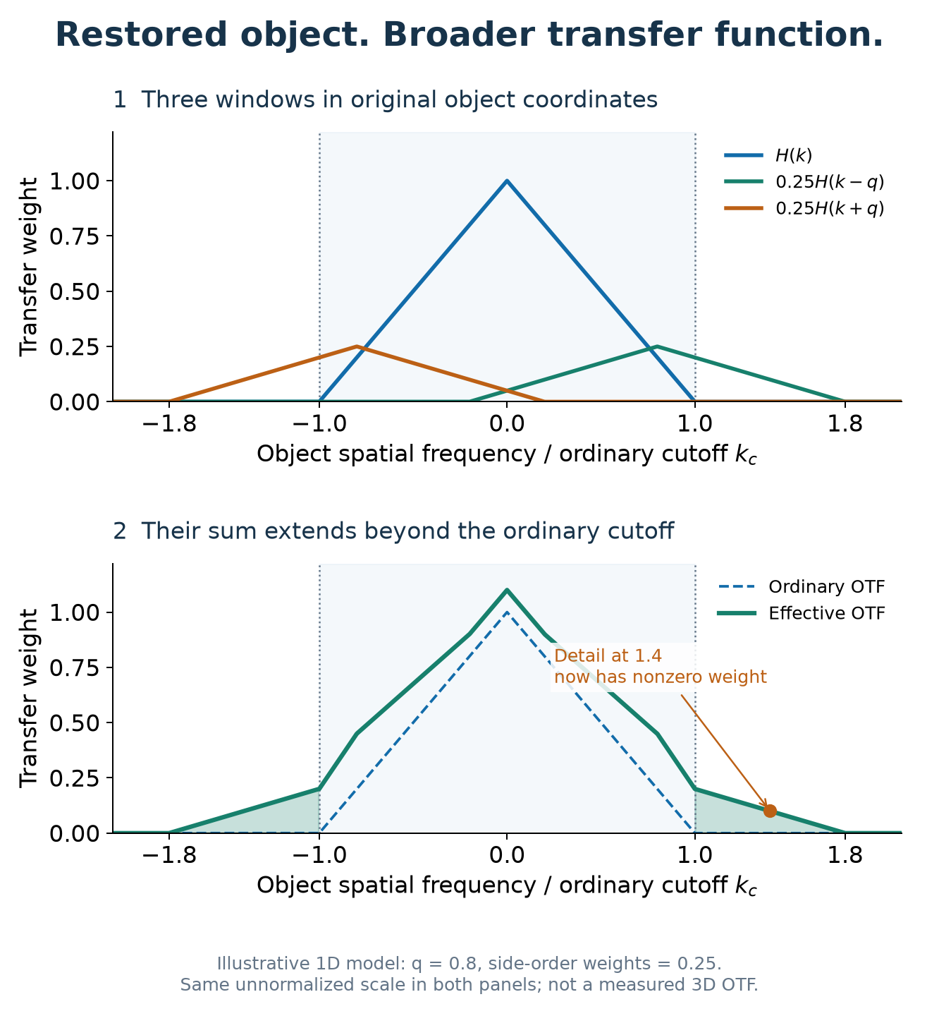 Figure 2. Adding the central and two shifted OTF windows extends the transfer range. This illustrative 1D model uses q = 0.8 and side-order weights of 0.25; it is not the instrument's measured 3D OTF.
In 3D, these shifts are vectors with lateral and axial components. The paper derives the scan averaging and numerically evaluates the rotating-system OTF, showing bandwidth extension in both directions and filling of the wide-field missing cone. See Section 2 and Figures 3–4 for the full mechanism.
4. What the experiment revealed
Using nominally 100 nm fluorescent beads, the paper reports these fitted image widths (FWHM):
| Direction | Wide-field | Spinning-disk 3D SIM |
|---|---|---|
| Lateral | 261 ± 11 nm | 129 ± 3 nm |
| Axial | 771 ± 47 nm | 388 ± 13 nm |
The SIM images were Wiener filtered; the wide-field comparison used raw images. Optical reconstruction replaces the conventional phase/orientation reconstruction workflow, while filtering enhances weak high-frequency detail.
The biological demonstration imaged ryanodine-receptor clusters inside a fixed rat cardiac cell approximately 12 µm thick, including a plane 6 µm below its surface. Nearby clusters that merged in wide-field images became distinguishable with spinning-disk 3D SIM. Figure 6 is the best place to see why the combination of resolution and background rejection matters.
These are results of the reported setup. Useful speed still depends on photon budget, a sufficiently uniform disk scan, and sample motion during the exposure; the fixed-cell experiment does not establish live-cell imaging at 100 frames/s.
5. See the full experiment
How does the eight-sector disk produce a uniform scan? Why does the lattice extend axial resolution? What do the improved cell images actually look like?
Read the open-access paper → Start with Figures 3–6 for the illumination, OTF, beads, and cell images; then follow Section 2 for the derivation and Section 3 for the optical design.
Youchang Zhang, Parisa Asghari, David R. L. Scriven, Edwin D. W. Moore, and Keng C. Chou. “3D structured illumination microscope using a spinning disk [Invited].” Biomedical Optics Express 14(11), 5710–5719 (2023). DOI: 10.1364/BOE.499181.