How a Silver Mirror Modifies Laser Polarization at 488 nm
On this page
Inspiration
This investigation grew out of a puzzle I encountered during my PhD while working on a structured illumination microscope, where precise control of the illumination polarization is essential. I converted a linearly polarized 488 nm laser beam into circularly polarized using an achromatic QWP, and verified it immediately after the QWP with an analyzer and power meter. However, after several mirror reflections and a beam-expanding telescope, the light reaching the microscope became elliptically polarized. I initially suspected it is due to an imperfect QWP, stress-induced lens birefringence, or contamination on the lens and mirrors.
The explanation became clear after I read P. C. Logofătu's paper, “Simple method for determining the fast axis of a wave plate”, which describes how a polished metal surface can introduce a phase shift between the and polarized components. It made me realize that the mirrors themselves, not necessarily defective optics, could have a significant effect on polarization - even transforming the circularly polarized beam into an linear one. That realization motivated the analysis presented here.
Summary
A mirror in a polarization-sensitive optical system is not merely a ray-folding element. At oblique incidence it is, more precisely, a lossy diattenuating retarder: it changes both the relative phase and the relative amplitude of the and polarized components.
For the worked example in this article,
and the incident medium is air, . The most useful numerical results are:
- The principal phase difference, , is at incidence and reaches at .
- Over the angular range considered here, runs from at normal incidence toward at grazing incidence, with the principal phase evaluated independently at each angle.
- Because silver is absorbing, there is no exact Brewster zero. The pseudo-Brewster angle, defined by the minimum of , is , where .
- The reflectance difference reaches about , or 2.95 percentage points, near .
- At , incident RCP or LCP light is reflected as an ellipse with , , and .
- At , both RCP and LCP input becomes linear in this ideal half-space model. The two input handednesses give linear states at orientations and .
Model scope and data source. The value is obtained by linear interpolation in wavelength at between the room-temperature Johnson–Christy silver samples and . It represents a semi-infinite silver half-space in this worked example, not every real mirror. Optical constants depend on film preparation and surface condition, while protected and finite-thickness mirrors require a multilayer model. See the Johnson–Christy data record and the refractiveindex.info database paper.
1. Geometry and conventions
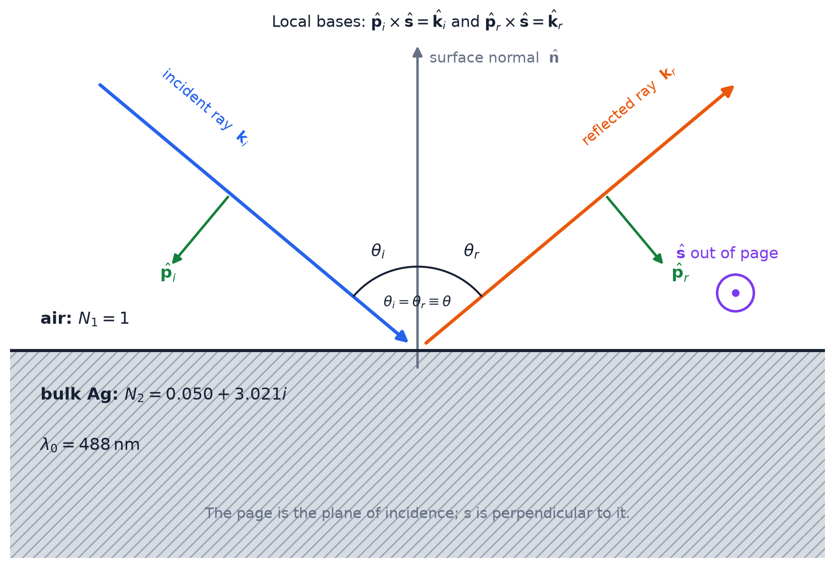 Incident and reflected rays at an air–silver interface, with the local s and p directions labeled
Figure 1. Reflection geometry and the local transverse bases used for the incident and reflected beams.
The interface is planar, the page is the plane of incidence, and the incidence angle is measured from the surface normal , which points from the silver into the air. Subscripts and mean incident and reflected, respectively.
Choose a single unit vector perpendicular to the plane of incidence and use it for both beams. The corresponding in-plane unit vectors are defined explicitly by
Thus and are right-handed local bases. Using the convention, the complex electric fields are
The reflected Jones vector is written in the reflected local basis:
Here, and are complex numbers. At normal incidence, . Because is kept fixed, the definitions above give . The resulting relation at is therefore a sign introduced by the two local coordinate frames, not an additional physical retardance of the mirror.
2. Mathematical model
2.1 Complex refraction and the physical square-root branch
Snell's law remains valid with a complex transmitted angle:
It is more convenient not to evaluate explicitly. Define the normalized normal component of the transmitted wavevector,
For the convention and a passive medium, choose the square-root branch with
so the field decays rather than grows inside the metal.
2.2 Fresnel coefficients
For incidence from air, the propagation-adapted Fresnel coefficients are
and
The reflected Jones matrix is therefore
Writing the two coefficients explicitly as and makes the two physical actions clear:
- produces diattenuation;
- describes their relative phase.
2.3 Jones vector to Stokes vector and ellipse
For a fully coherent reflected Jones vector
the Stokes parameters used here are
The ellipse orientation and signed ellipticity angle are
and
Equivalently, if
then the form used in the reference image is
The atan2 form should be used in code because it preserves the correct quadrant. The semi-axis lengths follow from
with
For the adopted time dependence, means that the field rotates counter-clockwise in a plot whose horizontal and vertical axes are and , respectively, as time advances.
3. Result: phase of the reflected and components
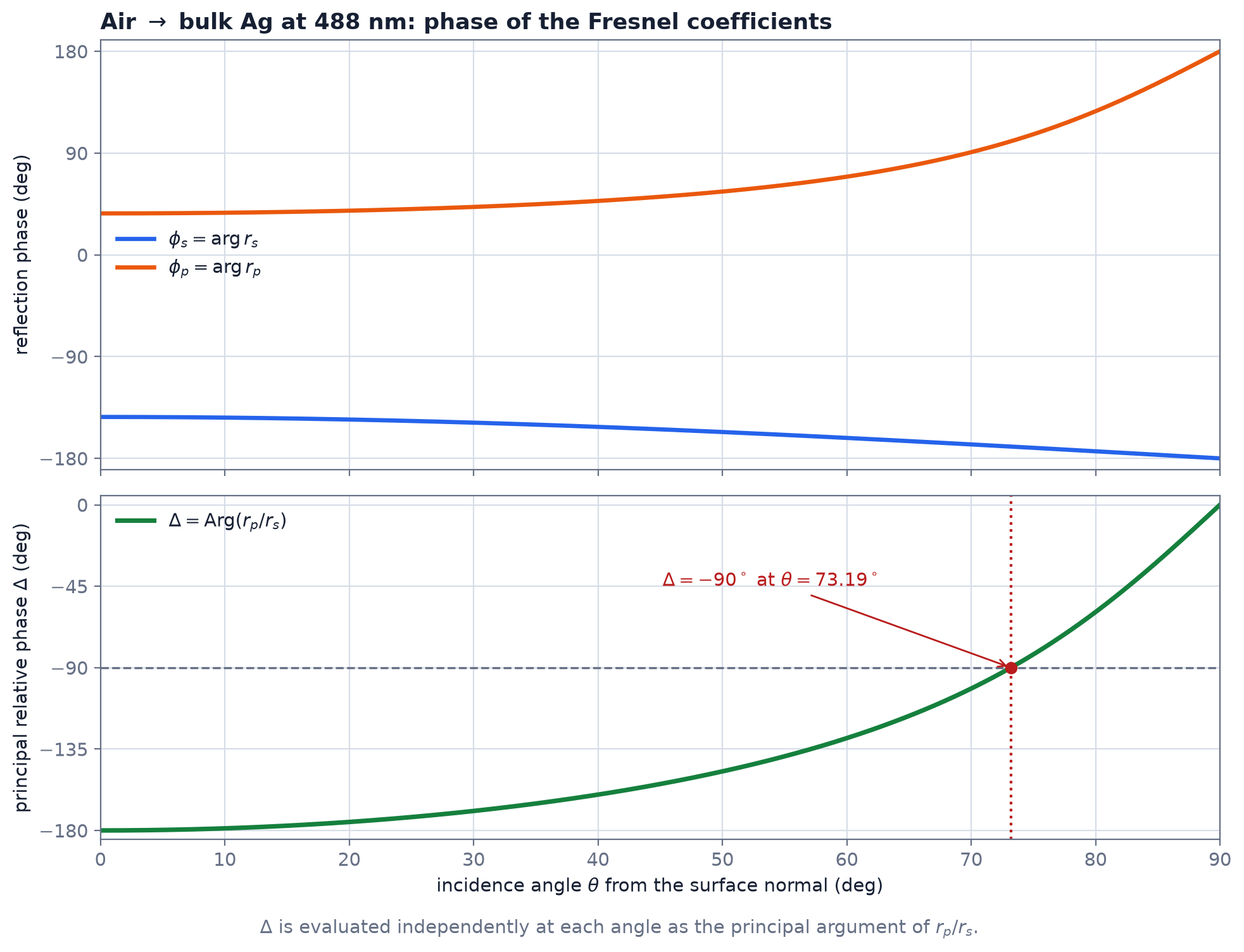 The s and p Fresnel reflection phases and their principal relative phase versus incidence angle
Figure 2. The individual reflection phases and the principal relative phase .
Define
Here denotes the argument of the complex number. The phase is calculated directly from the complex ratio at each angle. At normal incidence, is equivalent to .
| Incidence | |||
|---|---|---|---|
| () | |||
At , , so is purely negative imaginary and the two reflection coefficients are in quadrature. The interface is not an ideal quarter-wave plate, however, because ; its phase and amplitude effects must be considered together.
4. Result: power reflectance and the pseudo-Brewster angle
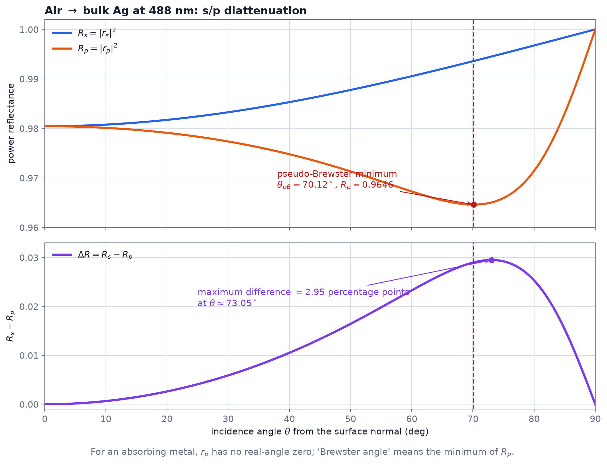 The s and p power reflectances and their difference versus incidence angle
Figure 3. Power reflectance and s/p diattenuation.
The power reflectances are
because the incident and reflected waves occupy the same medium. For a lossless dielectric, can cross zero at a real Brewster angle. For absorbing silver, is complex and does not vanish at any real angle. Here “Brewster angle” therefore means the pseudo-Brewster angle
| Incidence | ||||
|---|---|---|---|---|
| 0.98044 | 0.98044 | 0.00000 | 0.98044 | |
| 0.98117 | 0.97970 | 0.00147 | 0.98044 | |
| 0.98327 | 0.97737 | 0.00590 | 0.98032 | |
| 0.98649 | 0.97317 | 0.01332 | 0.97983 | |
| 0.99055 | 0.96727 | 0.02328 | 0.97891 | |
| (pseudo-Brewster) | 0.99361 | 0.96462 | 0.02899 | 0.97911 |
| 0.99457 | 0.96510 | 0.02947 | 0.97983 | |
| 0.99514 | 0.96594 | 0.02921 | 0.98054 | |
| 0.99837 | 0.98304 | 0.01533 | 0.99070 | |
| 0.99967 | 0.99637 | 0.00330 | 0.99802 | |
| 1.00000 | 1.00000 | 0.00000 | 1.00000 |
The largest amplitude discrimination does not occur exactly at the pseudo-Brewster angle. In this model, peaks near , where the difference is about 0.02948. Thus an oblique silver mirror is simultaneously a retarder and a diattenuator, although the diattenuation is modest for this 488 nm example.
5. Result: the reflected polarization when use RCP and LCP incidence
Circular-polarization labels vary between communities, so the Jones vectors are the definitive convention in this article. Looking toward the source, and using the local right-handed basis,
They have equal and amplitudes. Reflection gives
For either input handedness, the reflected component-amplitude ratio is
The component ratios are
Therefore their principal component phase differences are
5.1 Worked example at
At ,
Therefore
Both have total reflected power . Their ellipse shapes are identical and their orientations and handedness signs are mirror images:
| Input | ||||
|---|---|---|---|---|
| RCP, | 0.6288 | +0.9013 | ||
| LCP, | 0.6288 | -0.9013 |
For fully polarized light, is the normalized circular Stokes component: the power imbalance between the two circular basis states, divided by the total power. With the convention and the plotted axes, a positive value means counter-clockwise field rotation and a negative value means clockwise rotation. Its magnitude is 1 for circular polarization and 0 for linear polarization. Thus the values describe equally elliptical states with opposite rotation senses and ; they do not mean that 90.13% of the reflected power is “circular.”
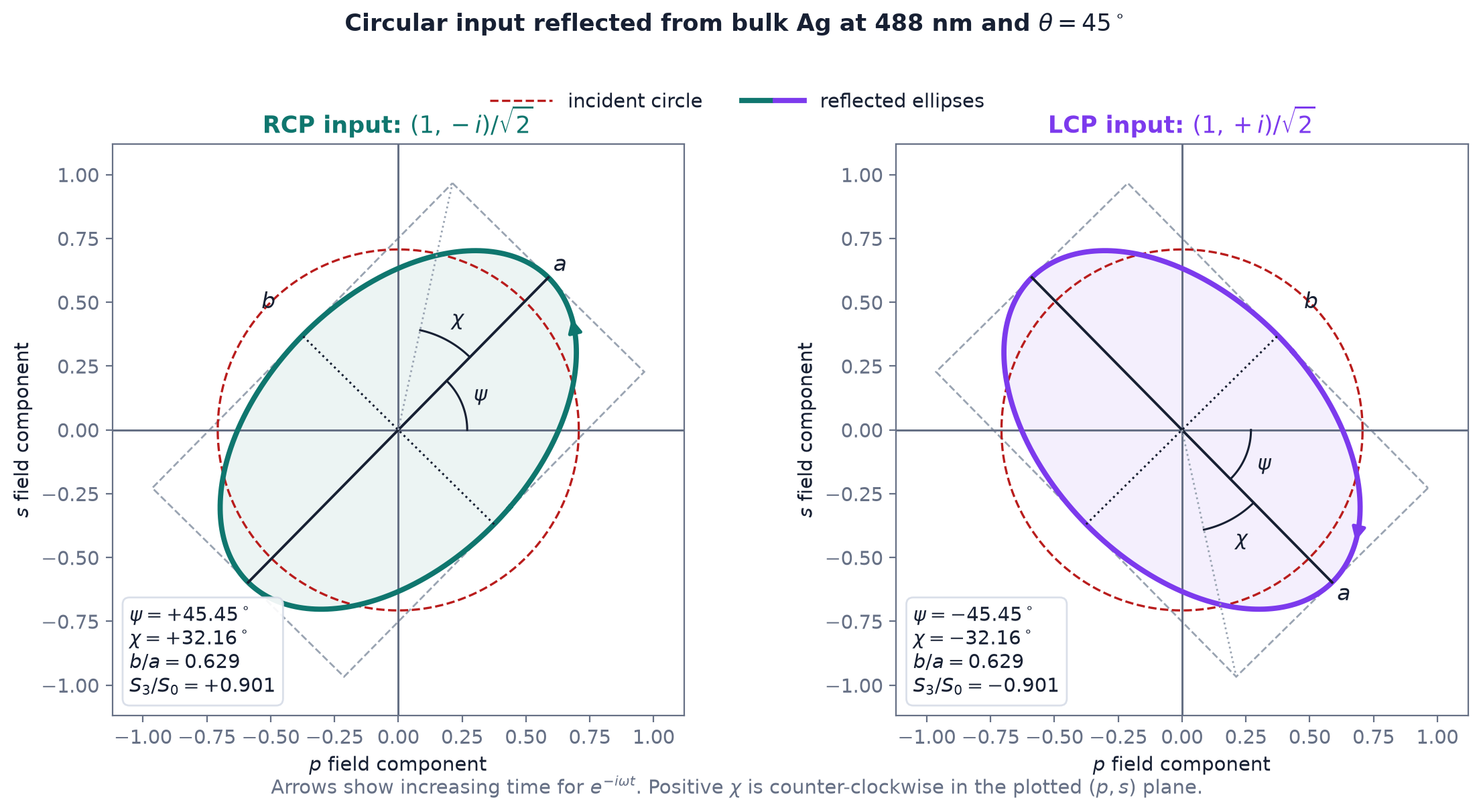 Reflected polarization ellipses for RCP and LCP input at 45 degrees
Figure 4. Reflected polarization ellipses at . The dashed circle is the incident circular locus; the arrows show increasing time. The auxiliary arc satisfies , and its sign follows the direction of field rotation.
5.2 Evolution with incidence angle
| 0.9553 | |||||
| 0.8277 | |||||
| 0.6288 | |||||
| 0.3538 | |||||
| 0.0978 | |||||
| 0.0000 | |||||
| 0.0639 | |||||
| 0.5633 |
Three limiting cases are worth remembering:
- Normal incidence: , so circular input remains circular, but its handedness sign reverses in the reflected local basis.
- : . Both circular inputs become linear, at opposite orientations.
- Grazing incidence: , , and . The output approaches circular again with the same local handedness sign as the input.
6. Design implications
- Treat each oblique mirror as a complex Jones element, not a simple ray reflector.
- Track the local bases through every fold; a basis-sign error can produce a false retardance or reverse the inferred handedness.
- Use the coating stack actually present in the instrument. A protective dielectric layer can change both phase and diattenuation substantially.
- In a multi-mirror system, multiply the Jones matrices together with the coordinate rotations between successive planes of incidence.
The central idea is simple: when polarization matters, every mirror deserves attention - each one acts like a wave plate in its effect on phase.
7. Supporting information
The standalone script requires NumPy and Matplotlib:
python -m pip install numpy matplotlib
python scripts/silver_mirror_polarization_488nm_v4.py
It regenerates all PNG/SVG figures and prints the three tables. The complete source is included below:
Show the complete Python source
#!/usr/bin/env python3
"""Reproduce the 488 nm silver-mirror polarization figures and tables.

Model
-----
* vacuum wavelength: 488 nm
* incident medium: air, n1 = 1
* reflecting half-space: bulk Ag, N = 0.05000 + 3.02077143j
* complex-field convention: E0 exp[i k.r - i omega t]
* local transverse basis: (p, s, k) is right-handed for each ray

The silver index is linearly interpolated at 0.488 um from the Johnson-Christy
samples (0.4714 um, 0.05, 2.869) and (0.4959 um, 0.05, 3.093).

The program writes both SVG and PNG figures to ../figures and prints the
Markdown tables used in the accompanying article.
"""

from __future__ import annotations

from pathlib import Path

import matplotlib as mpl

mpl.use("Agg")

import matplotlib.pyplot as plt
from matplotlib.legend_handler import HandlerTuple
from matplotlib.patches import Arc, FancyArrowPatch, Polygon, Rectangle
import numpy as np


WAVELENGTH_NM = 488.0
N_AIR = 1.0
N_AG = 0.05 + 3.0207714285714284j

ROOT = Path(__file__).resolve().parents[1]
FIGURE_DIR = ROOT / "figures"

BLUE = "#2563eb"
ORANGE = "#ea580c"
GREEN = "#15803d"
PURPLE = "#7c3aed"
TEAL = "#0f766e"
RED = "#b91c1c"
INK = "#172033"
MUTED = "#667085"
GRID = "#d7dde8"
SILVER = "#d7dce3"


def apply_plot_style() -> None:
    """Set a clean, website-friendly Matplotlib style."""

    mpl.rcParams.update(
        {
            "figure.facecolor": "white",
            "axes.facecolor": "white",
            "savefig.facecolor": "white",
            "font.family": "DejaVu Sans",
            "font.size": 10.5,
            "axes.labelcolor": INK,
            "axes.edgecolor": MUTED,
            "axes.titlecolor": INK,
            "xtick.color": MUTED,
            "ytick.color": MUTED,
            "text.color": INK,
            "grid.color": GRID,
            "grid.linewidth": 0.8,
            "legend.frameon": False,
            "svg.fonttype": "none",
        }
    )


def physical_sqrt(z: np.ndarray | complex) -> np.ndarray | complex:
    """Square root with the passive-medium branch Im(sqrt(z)) >= 0."""

    q = np.sqrt(z + 0j)
    return np.where(np.imag(q) < 0.0, -q, q)


def fresnel(theta_deg: np.ndarray | float) -> tuple[np.ndarray, np.ndarray]:
    """Return (r_s, r_p) in propagation-adapted local bases.

    q = N_Ag cos(theta_t) is the normalized transmitted normal wavevector.
    The formulas are specialized to n1 = 1.
    """

    theta = np.deg2rad(theta_deg)
    sin_theta = np.sin(theta)
    cos_theta = np.cos(theta)
    q = physical_sqrt(N_AG**2 - sin_theta**2)

    r_s = (cos_theta - q) / (cos_theta + q)
    r_p = (N_AG**2 * cos_theta - q) / (N_AG**2 * cos_theta + q)
    return r_s, r_p


def principal_phase_deg(z: np.ndarray | complex) -> np.ndarray | float:
    """Principal complex argument in the interval [-180, 180) degrees."""

    phase = (np.rad2deg(np.angle(z)) + 180.0) % 360.0 - 180.0
    phase = np.where(np.isclose(phase, 0.0, atol=1e-12, rtol=0.0), 0.0, phase)
    return phase


def phase_curves(theta_deg: np.ndarray) -> tuple[np.ndarray, np.ndarray, np.ndarray]:
    """Return principal phi_s, phi_p, and Delta = Arg(r_p/r_s) in degrees."""

    r_s, r_p = fresnel(theta_deg)
    phi_s = np.rad2deg(np.angle(r_s))
    phi_p = np.rad2deg(np.angle(r_p))
    relative_phase = principal_phase_deg(r_p / r_s)
    return phi_s, phi_p, relative_phase


def scalar_results(theta_deg: float) -> dict[str, float | complex]:
    """Fresnel phases and reflectances at one angle."""

    r_s_arr, r_p_arr = fresnel(theta_deg)
    r_s = complex(r_s_arr)
    r_p = complex(r_p_arr)
    phi_s = np.rad2deg(np.angle(r_s))
    phi_p = np.rad2deg(np.angle(r_p))
    relative_phase = float(principal_phase_deg(r_p / r_s))
    return {
        "r_s": r_s,
        "r_p": r_p,
        "phi_s": phi_s,
        "phi_p": phi_p,
        "relative_phase": relative_phase,
        "R_s": abs(r_s) ** 2,
        "R_p": abs(r_p) ** 2,
        "difference": abs(r_s) ** 2 - abs(r_p) ** 2,
    }


def golden_minimum(function, lower: float, upper: float, tolerance: float = 1e-11) -> float:
    """Dependency-free bounded scalar minimization."""

    ratio = (np.sqrt(5.0) - 1.0) / 2.0
    c = upper - ratio * (upper - lower)
    d = lower + ratio * (upper - lower)
    fc = function(c)
    fd = function(d)
    while upper - lower > tolerance:
        if fc < fd:
            upper, d, fd = d, c, fc
            c = upper - ratio * (upper - lower)
            fc = function(c)
        else:
            lower, c, fc = c, d, fd
            d = lower + ratio * (upper - lower)
            fd = function(d)
    return 0.5 * (lower + upper)


def pseudo_brewster_angle() -> float:
    """Angle at which R_p is minimized (there is no exact zero for complex N)."""

    def objective(theta_deg: float) -> float:
        _, r_p = fresnel(theta_deg)
        return float(abs(complex(r_p)) ** 2)

    return golden_minimum(objective, 0.0, 89.999999)


def maximum_diattenuation_angle() -> float:
    """Angle that maximizes R_s - R_p."""

    def objective(theta_deg: float) -> float:
        result = scalar_results(theta_deg)
        return -float(result["difference"])

    return golden_minimum(objective, 0.0, 89.999999)


def angle_for_relative_phase(target_deg: float, lower: float, upper: float) -> float:
    """Bisection solution for a selected principal relative phase."""

    def relative_phase_at(theta_deg: float) -> float:
        return float(scalar_results(theta_deg)["relative_phase"])

    for _ in range(100):
        middle = 0.5 * (lower + upper)
        if relative_phase_at(middle) < target_deg:
            lower = middle
        else:
            upper = middle
    return 0.5 * (lower + upper)


def reflected_jones(theta_deg: float, handedness: int) -> np.ndarray:
    """Jones vector [E_p, E_s] after reflection of circular input.

    handedness = -1: RCP input [1, -i]/sqrt(2)
    handedness = +1: LCP input [1, +i]/sqrt(2)
    """

    r_s, r_p = fresnel(theta_deg)
    return np.array([complex(r_p), 1j * handedness * complex(r_s)]) / np.sqrt(2.0)


def ellipse_metrics(jones: np.ndarray) -> dict[str, float]:
    """Return Stokes parameters and polarization-ellipse quantities.

    S3 = 2 Im(E_s E_p*) is consistent with exp(-i omega t). Positive chi
    therefore means counter-clockwise rotation in the plotted (p, s) plane.
    """

    e_p, e_s = jones
    s0 = abs(e_p) ** 2 + abs(e_s) ** 2
    s1 = abs(e_p) ** 2 - abs(e_s) ** 2
    s2 = 2.0 * np.real(e_p * np.conj(e_s))
    s3 = 2.0 * np.imag(e_s * np.conj(e_p))
    linear_part = np.hypot(s1, s2)
    psi = 0.5 * np.rad2deg(np.arctan2(s2, s1))
    chi = 0.5 * np.rad2deg(np.arcsin(np.clip(s3 / s0, -1.0, 1.0)))
    semi_major = np.sqrt(0.5 * (s0 + linear_part))
    semi_minor = np.sqrt(max(0.0, 0.5 * (s0 - linear_part)))
    return {
        "S0": float(s0),
        "S1": float(s1),
        "S2": float(s2),
        "S3": float(s3),
        "psi": float(psi),
        "chi": float(chi),
        "a": float(semi_major),
        "b": float(semi_minor),
        "b_over_a": float(semi_minor / semi_major),
    }


def save_figure(fig: plt.Figure, stem: str) -> None:
    """Save one figure in scalable and broadly compatible formats."""

    FIGURE_DIR.mkdir(parents=True, exist_ok=True)
    fig.savefig(FIGURE_DIR / f"{stem}.svg", bbox_inches="tight")
    fig.savefig(FIGURE_DIR / f"{stem}.png", dpi=200, bbox_inches="tight")
    plt.close(fig)


def draw_geometry() -> None:
    """Draw the incidence geometry and local p/s bases."""

    fig, ax = plt.subplots(figsize=(10.5, 5.8))
    ax.set_xlim(-5.1, 5.1)
    ax.set_ylim(-2.6, 4.2)
    ax.set_aspect("equal")
    ax.axis("off")

    ax.add_patch(Rectangle((-5.1, -2.6), 10.2, 2.6, facecolor=SILVER, edgecolor="none"))
    ax.add_patch(Rectangle((-5.1, -2.6), 10.2, 2.6, facecolor="none", edgecolor="#9aa4b2", hatch="///", linewidth=0.0))
    ax.plot([-5.1, 5.1], [0.0, 0.0], color=INK, lw=2.2)

    arrow = dict(arrowstyle="-|>", mutation_scale=16, lw=2.4)
    ax.add_patch(FancyArrowPatch((-4.0, 3.35), (-0.08, 0.07), color=BLUE, **arrow))
    ax.add_patch(FancyArrowPatch((0.08, 0.07), (4.0, 3.35), color=ORANGE, **arrow))
    ax.add_patch(FancyArrowPatch((0.0, -0.25), (0.0, 3.85), color=MUTED, arrowstyle="-|>", mutation_scale=14, lw=1.7))

    ax.text(-2.65, 2.52, r"incident ray  $\mathbf{k}_i$", color=BLUE, rotation=-40, ha="center", va="bottom")
    ax.text(2.65, 2.52, r"reflected ray  $\mathbf{k}_r$", color=ORANGE, rotation=40, ha="center", va="bottom")
    ax.text(0.15, 3.67, r"surface normal  $\hat{\mathbf{n}}$", color=MUTED, va="center")

    ray_angle = np.rad2deg(np.arctan2(3.35, 4.0))
    ax.add_patch(Arc((0, 0), 2.1, 2.1, theta1=ray_angle, theta2=90, color=INK, lw=1.4))
    ax.add_patch(Arc((0, 0), 2.1, 2.1, theta1=90, theta2=180 - ray_angle, color=INK, lw=1.4))
    ax.text(-0.58, 1.18, r"$\theta_i$", fontsize=12)
    ax.text(0.58, 1.18, r"$\theta_r$", fontsize=12)
    ax.text(0.0, 0.55, r"$\theta_i=\theta_r\equiv\theta$", ha="center", fontsize=10)

    # Propagation-adapted p vectors: p = s x k. Both lie in the page.
    p_style = dict(arrowstyle="-|>", mutation_scale=13, lw=1.8, color=GREEN)
    ax.add_patch(FancyArrowPatch((-2.35, 1.95), (-3.10, 1.05), **p_style))
    ax.add_patch(FancyArrowPatch((2.35, 1.95), (3.10, 1.05), **p_style))
    ax.text(-3.22, 0.91, r"$\hat{\mathbf{p}}_i$", color=GREEN, fontsize=12)
    ax.text(3.18, 0.91, r"$\hat{\mathbf{p}}_r$", color=GREEN, fontsize=12)

    # A circled dot denotes +s out of the page.
    s_x, s_y = 3.98, 0.72
    ax.add_patch(plt.Circle((s_x, s_y), 0.23, facecolor="white", edgecolor=PURPLE, lw=1.8))
    ax.plot([s_x], [s_y], marker="o", ms=4.5, color=PURPLE)
    ax.text(s_x - 0.10, s_y + 0.43, r"$\hat{\mathbf{s}}$ out of page", color=PURPLE, ha="center", fontsize=11)

    ax.text(-4.72, 0.33, r"air: $N_1=1$", fontsize=12, weight="bold")
    ax.text(-4.72, -0.62, rf"bulk Ag: $N_2={N_AG.real:.3f}+{N_AG.imag:.3f}i$", fontsize=12, weight="bold")
    ax.text(-4.72, -1.25, rf"$\lambda_0={WAVELENGTH_NM:.0f}\,\mathrm{{nm}}$", fontsize=12)
    ax.text(0.0, -2.10, "The page is the plane of incidence; s is perpendicular to it.", ha="center", color=MUTED)
    ax.text(
        0.0,
        4.05,
        r"Local bases: $\hat{\mathbf{p}}_i\times\hat{\mathbf{s}}=\hat{\mathbf{k}}_i$ and $\hat{\mathbf{p}}_r\times\hat{\mathbf{s}}=\hat{\mathbf{k}}_r$",
        ha="center",
        fontsize=11,
    )
    fig.tight_layout()
    save_figure(fig, "silver_reflection_geometry_488nm_v4")


def draw_phase_plot(theta_linear: float) -> None:
    """Plot principal reflection phases and their principal relative phase."""

    theta = np.linspace(0.0, 90.0, 1801)
    phi_s, phi_p, relative_phase = phase_curves(theta)

    fig, axes = plt.subplots(2, 1, figsize=(10.0, 7.5), sharex=True, gridspec_kw={"height_ratios": [1.25, 1.0]})
    ax0, ax1 = axes
    ax0.plot(theta, phi_s, color=BLUE, lw=2.4, label=r"$\phi_s=\arg r_s$")
    ax0.plot(theta, phi_p, color=ORANGE, lw=2.4, label=r"$\phi_p=\arg r_p$")
    ax0.set_ylabel("reflection phase (deg)")
    ax0.set_ylim(-190, 190)
    ax0.set_yticks([-180, -90, 0, 90, 180])
    ax0.grid(True)
    ax0.legend(loc="center left")
    ax0.set_title(rf"Air $\rightarrow$ bulk Ag at {WAVELENGTH_NM:.0f} nm: phase of the Fresnel coefficients", loc="left", weight="bold")

    ax1.plot(theta, relative_phase, color=GREEN, lw=2.6, label=r"$\Delta=\operatorname{Arg}(r_p/r_s)$")
    ax1.axhline(-90.0, color=MUTED, ls="--", lw=1.2)
    ax1.axvline(theta_linear, color=RED, ls=":", lw=1.5)
    ax1.plot([theta_linear], [-90.0], marker="o", color=RED, ms=6)
    ax1.annotate(
        rf"$\Delta=-90^\circ$ at $\theta={theta_linear:.2f}^\circ$",
        xy=(theta_linear, -90.0),
        xytext=(theta_linear - 28, -45),
        arrowprops={"arrowstyle": "->", "color": RED},
        color=RED,
    )
    ax1.set_xlabel(r"incidence angle $\theta$ from the surface normal (deg)")
    ax1.set_ylabel(r"principal relative phase $\Delta$ (deg)")
    ax1.set_xlim(0, 90)
    ax1.set_ylim(-185, 5)
    ax1.set_yticks([-180, -135, -90, -45, 0])
    ax1.grid(True)
    ax1.legend(loc="upper left")
    fig.text(0.5, 0.008, r"$\Delta$ is evaluated independently at each angle as the principal argument of $r_p/r_s$.", ha="center", color=MUTED)
    fig.tight_layout(rect=(0, 0.025, 1, 1))
    save_figure(fig, "silver_phase_vs_incidence_488nm_v4")


def draw_reflectance_plot(theta_pb: float) -> None:
    """Plot R_s, R_p and their difference."""

    theta = np.linspace(0.0, 90.0, 1801)
    r_s, r_p = fresnel(theta)
    r_s_power = abs(r_s) ** 2
    r_p_power = abs(r_p) ** 2
    difference = r_s_power - r_p_power
    theta_max = maximum_diattenuation_angle()
    maximum = scalar_results(theta_max)["difference"]

    fig, axes = plt.subplots(2, 1, figsize=(10.0, 7.5), sharex=True, gridspec_kw={"height_ratios": [1.25, 1.0]})
    ax0, ax1 = axes
    ax0.plot(theta, r_s_power, color=BLUE, lw=2.4, label=r"$R_s=|r_s|^2$")
    ax0.plot(theta, r_p_power, color=ORANGE, lw=2.4, label=r"$R_p=|r_p|^2$")
    ax0.axvline(theta_pb, color=RED, ls="--", lw=1.4)
    pb = scalar_results(theta_pb)
    ax0.plot([theta_pb], [pb["R_p"]], marker="o", color=RED, ms=6)
    ax0.annotate(
        "pseudo-Brewster minimum\n"
        + rf"$\theta_{{pB}}={theta_pb:.2f}^\circ$, $R_p={pb['R_p']:.4f}$",
        xy=(theta_pb, pb["R_p"]),
        xytext=(38, 0.968),
        arrowprops={"arrowstyle": "->", "color": RED},
        color=RED,
    )
    ax0.set_ylabel("power reflectance")
    ax0.set_ylim(0.960, 1.002)
    ax0.set_yticks([0.96, 0.97, 0.98, 0.99, 1.00])
    ax0.grid(True)
    ax0.legend(loc="upper left")
    ax0.set_title(rf"Air $\rightarrow$ bulk Ag at {WAVELENGTH_NM:.0f} nm: s/p diattenuation", loc="left", weight="bold")

    ax1.plot(theta, difference, color=PURPLE, lw=2.6, label=r"$\Delta R=R_s-R_p$")
    ax1.axvline(theta_pb, color=RED, ls="--", lw=1.4)
    ax1.plot([theta_max], [maximum], marker="o", color=PURPLE, ms=6)
    ax1.annotate(
        rf"maximum difference $={100*maximum:.2f}$ percentage points"
        + "\n"
        + rf"at $\theta\approx{theta_max:.2f}^\circ$",
        xy=(theta_max, maximum),
        xytext=(25, 0.020),
        arrowprops={"arrowstyle": "->", "color": PURPLE},
        color=PURPLE,
    )
    ax1.set_xlabel(r"incidence angle $\theta$ from the surface normal (deg)")
    ax1.set_ylabel(r"$R_s-R_p$")
    ax1.set_xlim(0, 90)
    ax1.set_ylim(-0.001, 0.033)
    ax1.set_yticks([0.00, 0.01, 0.02, 0.03])
    ax1.grid(True)
    ax1.legend(loc="upper left")
    fig.text(0.5, 0.008, r"For an absorbing metal, $r_p$ has no real-angle zero; 'Brewster angle' means the minimum of $R_p$.", ha="center", color=MUTED)
    fig.tight_layout(rect=(0, 0.025, 1, 1))
    save_figure(fig, "silver_reflectance_vs_incidence_488nm_v4")


def draw_ellipse_panel(ax: plt.Axes, theta_deg: float, label: str, handedness: int, color: str) -> None:
    """Draw one reflected polarization ellipse with axes and handedness arrow."""

    jones = reflected_jones(theta_deg, handedness)
    metrics = ellipse_metrics(jones)
    tau = np.linspace(0.0, 2.0 * np.pi, 721)
    e_p = np.real(jones[0]) * np.cos(tau) + np.imag(jones[0]) * np.sin(tau)
    e_s = np.real(jones[1]) * np.cos(tau) + np.imag(jones[1]) * np.sin(tau)

    ax.axhline(0.0, color=MUTED, lw=1.1)
    ax.axvline(0.0, color=MUTED, lw=1.1)
    circle_t = np.linspace(0.0, 2.0 * np.pi, 361)
    input_radius = 1.0 / np.sqrt(2.0)
    ax.plot(input_radius * np.cos(circle_t), input_radius * np.sin(circle_t), color=RED, ls="--", lw=1.2, label="incident circle")
    ax.plot(e_p, e_s, color=color, lw=2.8, label="reflected ellipse")
    ax.fill(e_p, e_s, color=color, alpha=0.08)

    psi_rad = np.deg2rad(metrics["psi"])
    major = np.array([np.cos(psi_rad), np.sin(psi_rad)])
    minor = np.array([-np.sin(psi_rad), np.cos(psi_rad)])
    a = metrics["a"]
    b = metrics["b"]
    ax.plot([-a * major[0], a * major[0]], [-a * major[1], a * major[1]], color=INK, lw=1.4)
    ax.plot([-b * minor[0], b * minor[0]], [-b * minor[1], b * minor[1]], color=INK, lw=1.1, ls=":")
    corners = np.array(
        [
            a * major + b * minor,
            a * major - b * minor,
            -a * major - b * minor,
            -a * major + b * minor,
        ]
    )
    ax.add_patch(Polygon(corners, closed=True, fill=False, edgecolor="#9aa4b2", lw=1.0, ls="--"))

    ax.text(*(1.08 * a * major), r"$a$", color=INK, fontsize=12, ha="center", va="center")
    ax.text(*(1.35 * b * minor), r"$b$", color=INK, fontsize=12, ha="center", va="center")
    psi_arc = np.linspace(0.0, psi_rad, 80)
    radius = 0.27
    ax.plot(radius * np.cos(psi_arc), radius * np.sin(psi_arc), color=INK, lw=1.1)
    mid = 0.5 * psi_rad
    ax.text(0.35 * np.cos(mid), 0.35 * np.sin(mid), r"$\psi$", fontsize=11, ha="center", va="center")

    # The auxiliary triangle makes tan(|chi|) = b/a visible in the plot.
    chi_rad = np.deg2rad(metrics["chi"])
    chi_side = 1.0 if chi_rad >= 0.0 else -1.0
    chi_corner = a * major + chi_side * b * minor
    ax.plot([0.0, chi_corner[0]], [0.0, chi_corner[1]], color="#9aa4b2", lw=1.0, ls=":")
    chi_arc = np.linspace(psi_rad, psi_rad + chi_rad, 50)
    chi_radius = 0.40
    ax.plot(chi_radius * np.cos(chi_arc), chi_radius * np.sin(chi_arc), color=INK, lw=1.1)
    chi_mid = psi_rad + 0.5 * chi_rad
    ax.text(0.49 * np.cos(chi_mid), 0.49 * np.sin(chi_mid), r"$\chi$", fontsize=11, ha="center", va="center")

    # Arrow follows increasing physical time for the exp(-i omega t) convention.
    arrow_index = 118
    direction = FancyArrowPatch(
        (e_p[arrow_index], e_s[arrow_index]),
        (e_p[arrow_index + 13], e_s[arrow_index + 13]),
        arrowstyle="-|>",
        mutation_scale=15,
        lw=1.8,
        color=color,
    )
    ax.add_patch(direction)

    ax.set_xlim(-1.12, 1.12)
    ax.set_ylim(-1.12, 1.12)
    ax.set_aspect("equal")
    ax.set_xlabel(r"$p$ field component")
    ax.set_ylabel(r"$s$ field component")
    ax.set_title(label, color=color, weight="bold")
    ax.grid(False)
    ax.text(
        0.03,
        0.03,
        rf"$\psi={metrics['psi']:+.2f}^\circ$" + "\n" + rf"$\chi={metrics['chi']:+.2f}^\circ$" + "\n" + rf"$b/a={metrics['b_over_a']:.3f}$" + "\n" + rf"$S_3/S_0={metrics['S3']/metrics['S0']:+.3f}$",
        transform=ax.transAxes,
        va="bottom",
        bbox={"boxstyle": "round,pad=0.35", "facecolor": "white", "edgecolor": GRID, "alpha": 0.92},
    )


def draw_polarization_ellipses(theta_deg: float = 45.0) -> None:
    """Compare reflected RCP and LCP polarization ellipses."""

    fig, axes = plt.subplots(1, 2, figsize=(11.5, 5.8))
    draw_ellipse_panel(axes[0], theta_deg, r"RCP input: $(1,-i)/\sqrt{2}$", -1, TEAL)
    draw_ellipse_panel(axes[1], theta_deg, r"LCP input: $(1,+i)/\sqrt{2}$", +1, PURPLE)
    left_handles, _ = axes[0].get_legend_handles_labels()
    right_handles, _ = axes[1].get_legend_handles_labels()
    incident_handle = left_handles[0]
    reflected_handles = (left_handles[1], right_handles[1])
    fig.legend(
        [incident_handle, reflected_handles],
        ["incident circle", "reflected ellipses"],
        handler_map={tuple: HandlerTuple(ndivide=None, pad=0.2)},
        loc="upper center",
        ncol=2,
        bbox_to_anchor=(0.5, 0.93),
        handlelength=3.2,
    )
    fig.suptitle(rf"Circular input reflected from bulk Ag at {WAVELENGTH_NM:.0f} nm and $\theta={theta_deg:.0f}^\circ$", x=0.5, y=1.01, weight="bold")
    fig.text(0.5, 0.005, r"Arrows show increasing time for $e^{-i\omega t}$. Positive $\chi$ is counter-clockwise in the plotted $(p,s)$ plane.", ha="center", color=MUTED)
    fig.tight_layout(rect=(0, 0.035, 1, 0.94), w_pad=3.5)
    save_figure(fig, "silver_reflected_circular_ellipses_45deg_488nm_v4")


def print_markdown_tables(theta_pb: float, theta_linear: float) -> None:
    """Print the selected numerical results in Markdown table syntax."""

    selected = sorted([0.0, 15.0, 30.0, 45.0, 60.0, theta_pb, theta_linear, 75.0, 85.0, 89.0, 90.0])

    print("\nPHASE TABLE\n")
    print("| theta (deg) | phi_s (deg) | phi_p (deg) | Delta (deg) |")
    print("|---:|---:|---:|---:|")
    for theta in selected:
        result = scalar_results(theta)
        print(
            f"| {theta:0.2f} | {result['phi_s']:0.2f} | {result['phi_p']:0.2f} | "
            f"{result['relative_phase']:0.2f} |"
        )

    print("\nREFLECTANCE TABLE\n")
    print("| theta (deg) | R_s | R_p | R_s - R_p | mean reflectance |")
    print("|---:|---:|---:|---:|---:|")
    for theta in selected:
        result = scalar_results(theta)
        mean = 0.5 * (result["R_s"] + result["R_p"])
        print(
            f"| {theta:0.2f} | {result['R_s']:0.5f} | {result['R_p']:0.5f} | "
            f"{result['difference']:0.5f} | {mean:0.5f} |"
        )

    print("\nCIRCULAR-INPUT ELLIPSE TABLE\n")
    print("| theta (deg) | psi_R (deg) | chi_R (deg) | psi_L (deg) | chi_L (deg) | b/a |")
    print("|---:|---:|---:|---:|---:|---:|")
    for theta in sorted([15.0, 30.0, 45.0, 60.0, theta_pb, theta_linear, 75.0, 85.0]):
        right = ellipse_metrics(reflected_jones(theta, -1))
        left = ellipse_metrics(reflected_jones(theta, +1))
        print(
            f"| {theta:0.2f} | {right['psi']:+0.2f} | {right['chi']:+0.2f} | "
            f"{left['psi']:+0.2f} | {left['chi']:+0.2f} | {right['b_over_a']:0.4f} |"
        )


def main() -> None:
    apply_plot_style()
    theta_pb = pseudo_brewster_angle()
    theta_linear = angle_for_relative_phase(-90.0, 45.0, 75.0)
    draw_geometry()
    draw_phase_plot(theta_linear)
    draw_reflectance_plot(theta_pb)
    draw_polarization_ellipses(45.0)
    print(f"pseudo-Brewster angle = {theta_pb:.8f} deg")
    print(f"Delta = -90 deg angle = {theta_linear:.8f} deg")
    print_markdown_tables(theta_pb, theta_linear)


if __name__ == "__main__":
    main()
References
- P. C. Logofătu, “Simple method for determining the fast axis of a wave plate,” Optical Engineering 41(12), 3316–3318 (2002).
- M. N. Polyanskiy, “Refractiveindex.info database of optical constants,” Scientific Data 11, 94 (2024).
- P. B. Johnson and R. W. Christy, “Optical Constants of the Noble Metals,” Physical Review B 6, 4370–4379 (1972).