Pulsed Laser Generation: Mode Locking and Q-Switching

Inspiration

A few months ago, I had an interview with 中科飞测 (Skyverse Technology). During the interview, I was asked to explain how pulsed lasers work and describe the difference between Q-switching and mode locking.

Although I had studied both techniques before, years had passed that I had forgotten many details. That question motivated me to revisit the subject and organize my understanding more systematically.

This article is the result: a review of how mode locking and Q-switching work, how their principal specifications are calculated, and where each method is most useful. I hope it can also serve as a helpful introduction for anyone who wants to understand these two important approaches to pulse generation.

Short summary

A continuous-wave (CW) laser distributes its output energy continuously in time. A pulsed laser concentrates energy into short intervals, so its peak power can be far higher than its average power. Two of the most important methods of generating laser pulses are mode locking and Q-switching.

• Mode locking establishes a fixed phase relationship among many longitudinal cavity modes. Their coherent superposition produces an ultrashort pulse that circulates in the cavity.
• Q-switching suppresses laser oscillation while energy accumulates in the gain medium, then rapidly reduces the cavity loss and releases that energy in a short, energetic pulse.

Their typical specifications and applications reflect this difference:

These ranges are representative, not absolute. Amplified mode-locked systems, for example, can produce millijoule or even much higher pulse energies.

1. How mode locking works

1.1 Longitudinal modes of a laser cavity

A laser resonator (cavity) supports a discrete set of resonant optical frequencies called longitudinal modes. Only frequencies that reproduce their phase after a cavity round trip (constructive interference) can persist. For a simple linear cavity of physical length $L$, filled uniformly by a material of refractive index $n$, the resonant frequencies are approximately

$$\nu_m=m\frac{c}{2nL}.$$

Here, $\nu_m$ is the frequency of the $m$-th longitudinal mode, $m$ is a large integer mode number, and $c$ is the speed of light in vacuum. The product $nL$ is the one-way optical path length. In a cavity containing several materials, it is replaced by the sum of the optical path lengths of the individual sections.

The spacing between adjacent longitudinal modes is the free spectral range (FSR):

$$\boxed{ \mathrm{FSR}=\Delta\nu_{\mathrm{FSR}} =\frac{c}{2nL} =\frac{1}{T_{\mathrm{RT}}}}$$

In this expression, $\Delta\nu_{\mathrm{FSR}}=\nu_{m+1}-\nu_m$ is the mode spacing and $T_{\mathrm{RT}}=2nL/c$ is the cavity round-trip time.

For example, if the one-way optical path length $nL$ is $1.5\ \mathrm{m}$, then

$$\mathrm{FSR}\approx\frac{3.00\times10^8\ \mathrm{m/s}} {2(1.5\ \mathrm{m})}=100\ \mathrm{MHz}.$$

The cavity may therefore support modes at

$$\ldots,\quad \nu_0-100\ \mathrm{MHz},\quad \nu_0,\quad \nu_0+100\ \mathrm{MHz},\quad\ldots$$

where $\nu_0$ denotes the central optical frequency. The optical frequencies themselves may be hundreds of terahertz; $100\ \mathrm{MHz}$ is only their spacing.

1.2 From many longitudinal modes to one pulse

The intracavity electric field can be represented as a sum of longitudinal modes:

$$E(t)=\sum_m A_m \exp\!\left[i\left(2\pi\nu_m t+\phi_m\right)\right].$$

Here, $E(t)$ is the complex electric field at time $t$, $A_m$ is the amplitude of mode $m$, $\nu_m$ is its optical frequency, $\phi_m$ is its phase offset, and $i=\sqrt{-1}$. The measured optical intensity is proportional to $|E(t)|^2$.

If the phases $\phi_m$ fluctuate independently, the modes do not consistently reinforce one another at a particular time. The output is approximately continuous, with irregular intensity fluctuations.

The key idea of mode locking is:

$${\phi_m\text{ are locked relative to each other}}$$

For example,

$$\phi_m = \text{constant}$$

or, more generally, a fixed linear phase relation.

In a mode-locked laser, the phases have a fixed relationship. They do not have to be numerically identical; a linear phase progression from one mode to the next merely shifts the pulse in time. Once the relative phases are fixed, the fields interfere constructively during a short time interval and destructively during most of the remaining round trip. That creates a pulse.

1.3 How one pulse repeats to a pulse train

Consider three equally spaced modes with equal amplitudes and zero initial phase:

$$\nu_0,\qquad \nu_0+\Delta\nu_{\mathrm{FSR}},\qquad \nu_0+2\Delta\nu_{\mathrm{FSR}}.$$

Their combined field is

$$E(t)=e^{i2\pi\nu_0t} \left[1+e^{i2\pi\Delta\nu_{\mathrm{FSR}}t} +e^{i4\pi\Delta\nu_{\mathrm{FSR}}t}\right].$$

The leading factor $e^{i2\pi\nu_0t}$ is the rapid carrier phase oscillation. The bracketed factor represents a time-varying interference. At $t=0$, all three terms in brackets equal one and add up constructively. The exact same constructive interference occurs again after the repetition time $T_{\mathrm{rep}}$

$${T_{\mathrm{rep}}=\frac{1}{\Delta\nu_{\mathrm{FSR}}}=\frac{1}{\mathrm{FSR}}}$$

This is how the pulse repeats to a pulse train. This pulse train has a repetition rate of

$$\boxed{f_{\mathrm{rep}}=\frac{1}{T_{\mathrm{rep}}}=\Delta\nu_{\mathrm{FSR}}=\mathrm{FSR}=\frac{1}{T_{\mathrm{RT}}}}.$$

Fundamental mode locking produces one pulse per cavity round trip, so $f_{\mathrm{rep}}=\mathrm{FSR}$. Harmonic mode locking can produce an integer multiple of the FSR, while an external pulse picker can reduce the final delivered rate.

1.4 Active and passive mode locking

It is appealing to generate short, high-peak-power pulses by establishing a fixed phase relationship among the longitudinal modes. The next question is how to create and maintain that relationship. Based on the modulation mechanism, mode-locking methods can be categorized into active and passive techniques.

In active mode locking, an electro-optic modulator (EOM) or acousto-optic modulator (AOM) changes the cavity loss or phase periodically. When the modulation frequency matches the cavity round-trip frequency, or an integer multiple of it, light returning at the correct time experiences the same modulation on every round trip. This establishes a stable pulse train.

In passive mode locking, the cavity contains an intensity-dependent element. A common example is a saturable absorber: low-intensity light experiences more loss, while a sufficiently intense pulse partially bleaches the absorber and experiences less loss.

Both mechanisms favor short, intense pulses over a much weaker background of continuous spontaneous emission. They do not actively control the phase of each individual optical frequency component. Rather, they impose conditions under which only certain longitudinal modes—with fixed phase relationships—can build up coherently in the cavity. In other words, they do not independently modulate each frequency; they select which cavity modes are allowed to oscillate and, in the case of mode locking, enforce a stable phase relationship among those modes to form a high-intensity pulse.

1.5 Case study: Kerr-lens mode locking

Kerr-lens mode locking (KLM) is a passive mode locking technique. It relies on the optical Kerr effect:

$$n(I)=n_0+n_2 I.$$

Here, $n(I)$ is the intensity-dependent refractive index of the gain medium, $n_0$ is its low-intensity refractive index, $n_2$ is the nonlinear refractive-index coefficient, and $I$ is the local optical intensity. Because a beam is normally most intense near its axis, a positive $n_2$ produces a radial index profile that acts like a focusing lens. A high-intensity pulse therefore experiences a stronger Kerr lens than CW light.

Time sequence of a KLM oscillator:

1. Random fluctuations occasionally produce a brief intensity spike.
2. That spike creates a stronger Kerr lens than continuous-wave light.
3. The cavity is arranged so that the better-focused spike either:
   • passes through an aperture with lower loss (“hard-aperture” mode locking, see illustration below), or
   • overlaps the pumped gain region more effectively (“soft-aperture” mode locking).
4. The spike receives preferential amplification on each round trip.
5. Many longitudinal modes lock their phases together, forming a stable ultrashort pulse.

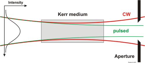Kerr-lens mode-locking schematic

Figure 1. Schematic of a hard-aperture KLM. The intense pulsed beam is focused more strongly than the CW beam and therefore experiences less aperture loss. Figure from Wikipedia. [1]

The Kerr response is effectively instantaneous on the timescale of a femtosecond pulse and does not require a separate absorbing element. These properties support pulses of <100 fs duration, broad bandwidth and high peak power. Demonstrated KLM Ti:sapphire oscillators include a 5 fs system with a spectrum extending from 600 to 1200 nm [2] and an extended-cavity chirped-pulse oscillator producing 220 nJ, 30 fs externally compressed pulses with peak power above 5 MW [3].

Note: The Kerr nonlinearity also produces self-phase modulation (SPM), which can broaden the optical spectrum. Dispersion of the gain medium also gives the new frequency components different group delays. Ordinary crystal materials around 800 nm usually contribute positive group-delay dispersion (GDD), which chirps and temporally broadens the pulse. Prism pairs, chirped mirrors, or other negative-GDD elements are therefore often used to balance the cavity dispersion. See section 1.7 for further discussion on GDD.

1.6 Typical mode-locked-laser specifications

(a) Repetition rate and cavity length

For a simple free-space linear cavity,

$$f_{\mathrm{rep}}\approx\frac{c}{2L}.$$

Here, $L$ is the one-way geometrical cavity length and the refractive index has been approximated as one. Equivalently,

$$L\approx\frac{c}{2f_{\mathrm{rep}}}.$$

For $f_{\mathrm{rep}}=80\ \mathrm{MHz}$,

$$T_{\mathrm{RT}}=\frac{1}{f_{\mathrm{rep}}} =12.5\ \mathrm{ns}, \qquad L\approx1.88\ \mathrm{m}.$$

Mirrors can fold this optical path so the laser occupies much less than $1.88\ \mathrm{m}$ of table length. Longer cavities have lower fundamental repetition rates; shorter cavities have higher rates.

(b) Pulse energy and average power

For a uniform train of identical pulses,

$$E_{\mathrm{pulse}}=\frac{P_{\mathrm{avg}}}{f_{\mathrm{rep}}}, \qquad P_{\mathrm{avg}}=E_{\mathrm{pulse}}f_{\mathrm{rep}}.$$

Here, $E_{\mathrm{pulse}}$ is the energy in one pulse and $P_{\mathrm{avg}}$ is the time-averaged output power. A $1\ \mathrm{W}$, $80\ \mathrm{MHz}$ laser therefore has

$$E_{\mathrm{pulse}} =\frac{1\ \mathrm{W}}{80\times10^6\ \mathrm{s^{-1}}} =12.5\ \mathrm{nJ}.$$

(c) Peak power, intensity, and fluence

The simplest peak-power estimate is

$$P_{\mathrm{peak}}\approx\frac{E_{\mathrm{pulse}}}{\tau_p},$$

where $P_{\mathrm{peak}}$ is the pulse's maximum instantaneous power and $\tau_p$ is a characteristic pulse duration. If $\tau_{\mathrm{FWHM}}$ is the full width at half maximum (FWHM) of the intensity profile, a more accurate expression is

$$P_{\mathrm{peak}}=K\frac{E_{\mathrm{pulse}}}{\tau_{\mathrm{FWHM}}}.$$

The dimensionless shape factor $K$ is approximately $0.94$ for a Gaussian intensity profile and $0.88$ for a $\operatorname{sech}^2$ profile. Thus, a $12.5\ \mathrm{nJ}$, $100\ \mathrm{fs}$ Gaussian pulse has

$$P_{\mathrm{peak}} \approx0.94\frac{12.5\ \mathrm{nJ}}{100\ \mathrm{fs}} \approx117\ \mathrm{kW}.$$

If $A_{\mathrm{eff}}$ is the effective illuminated area, useful first estimates are

$$I_{\mathrm{peak}}\approx\frac{P_{\mathrm{peak}}}{A_{\mathrm{eff}}}, \qquad F\approx\frac{E_{\mathrm{pulse}}}{A_{\mathrm{eff}}}.$$

Here, $I_{\mathrm{peak}}$ is peak intensity and $F$ is pulse fluence, or energy per unit area. Exact values depend on the spatial beam profile and on how the beam radius is defined.

(d) Optical bandwidth and pulse duration

A short pulse requires a broad optical spectrum. For an ideal transform-limited pulse,

$$\Delta\nu_{\mathrm{opt}}\,\tau_{\mathrm{FWHM}}=\mathrm{TBP}.$$

In this equation, $\Delta\nu_{\mathrm{opt}}$ is the FWHM bandwidth of the pulse's optical spectrum, $\tau_{\mathrm{FWHM}}$ is the FWHM intensity duration, and TBP is the dimensionless time–bandwidth product. With FWHM conventions,

$$\mathrm{TBP}=0.441\quad\text{for a Gaussian pulse}, \qquad \mathrm{TBP}=0.315\quad\text{for a }\operatorname{sech}^2\text{ pulse}.$$

For a non-transform-limited pulse the product is larger. Near a center wavelength $\lambda_0$, a small wavelength bandwidth $\Delta\lambda$ can be converted to frequency bandwidth by

$$\Delta\nu_{\mathrm{opt}}\approx \frac{c\,\Delta\lambda}{\lambda_0^2}, \qquad \Delta\lambda\ll\lambda_0.$$

Here, $\lambda_0$ is the center wavelength and $\Delta\lambda$ is the wavelength FWHM. A Gaussian pulse centered at $1030\ \mathrm{nm}$ with a $10\ \mathrm{nm}$ bandwidth has $\Delta\nu_{\mathrm{opt}}\approx2.83\ \mathrm{THz}$, giving a transform-limited duration of

$$\tau_{\mathrm{FWHM}} \approx\frac{0.441}{2.83\ \mathrm{THz}} \approx156\ \mathrm{fs}.$$

The approximate number of cavity modes inside this bandwidth is

$$N_{\mathrm{modes}}\approx \frac{\Delta\nu_{\mathrm{opt}}}{\Delta\nu_{\mathrm{FSR}}},$$

where $N_{\mathrm{modes}}$ is the mode count and $\Delta\nu_{\mathrm{FSR}}$ is the FSR. An $80\ \mathrm{MHz}$ oscillator using $2.83\ \mathrm{THz}$ of bandwidth therefore spans roughly $3.5\times10^4$ longitudinal modes. Their amplitudes are not equal in practice, and the pulse duration is determined by the complete spectral amplitude and phase, not by the mode count alone.

1.7 Dispersion and chirp

Mode locking can persist in a cavity with spectral dispersion, but dispersion makes different frequency components accumulate different phase delays. The pulse may remain stable while becoming temporally longer than its transform limit.

We can write the spectral electric field as

$$\tilde E(\omega)=A(\omega)e^{i\phi(\omega)}.$$

Here, $\tilde E(\omega)$ is the complex field as a function of angular frequency $\omega=2\pi\nu$, $A(\omega)$ is its spectral amplitude, and $\phi(\omega)$ is its spectral phase. Expanding the phase around the carrier angular frequency $\omega_0$ gives

$$\phi(\omega)=\phi_0+\phi_1(\omega-\omega_0) +\frac{1}{2}\phi_2(\omega-\omega_0)^2+\cdots.$$

The coefficient $\phi_0$ is an overall phase; $\phi_1=d\phi/d\omega|_{\omega_0}$ is a group delay and shifts the pulse in time; and

$$\phi_2=\left.\frac{d^2\phi}{d\omega^2}\right|_{\omega_0}=\mathrm{GDD}=\mathrm{GVD}\times d$$

where GDD is the group-delay dispersion, measured in units of $\mathrm{fs^2}$; GVD is the group-velocity dispersion, measured in units of $\mathrm{fs^2/mm}$; and $d$ is the propagation length through the material. Nonzero GDD creates a frequency-dependent group delay, normally chirping and broadening the pulse. Higher derivatives of $\phi$ produce more complicated temporal distortions.

For example, if a crystal has

$$\mathrm{GVD}=50\ \mathrm{fs^2/mm}$$

and the pulse travels through $4\ \mathrm{mm}$, then

$$\mathrm{GDD}=50\times4=200\ \mathrm{fs^2}.$$

For a transform-limited Gaussian pulse with initial pulse duration FWHM $\tau_0$, propagation through a purely quadratic spectral phase $\phi_2$ produces the duration [4]

$$\tau=\tau_0 \sqrt{1+\left(\frac{4\ln2\,\phi_2}{\tau_0^2}\right)^2}.$$

Here, $\tau$ is the broadened intensity FWHM and $\ln2$ is the natural logarithm of two. The equation assumes a Gaussian pulse, no higher-order dispersion, and no nonlinear propagation during the dispersive step.

Dispersion can be controlled with prism pairs, grating pairs, chirped mirrors, fibers, bulk materials, or combinations of these elements. In many modern mode-locked lasers, dispersion is deliberately designed together with SPM, gain, loss, and spectral filtering rather than simply being reduced to zero.

2. How Q-switching works

2.1 The cavity quality factor Q

The dimensionless quality factor $Q$ describes how slowly a passive cavity loses stored optical energy:

$$Q=\omega_0\tau_{\mathrm{cav}}.$$

Here, $\omega_0=2\pi\nu_0$ is the resonance angular frequency, $\nu_0$ is the corresponding ordinary frequency, and $\tau_{\mathrm{cav}}$ is the cold-cavity energy-decay time, often called the photon lifetime. “Cold cavity” means that gain or pump is ignored. If the stored energy is $U_0$ at $t=0$, it decays as

$$U(t)=U_0e^{-t/\tau_{\mathrm{cav}}},$$

where $U(t)$ is the energy remaining after time $t$. After one lifetime $\tau_{\mathrm{cav}}$, $U=U_0/e\approx0.368U_0$.

For a cavity resonance at $\lambda_0=800\ \mathrm{nm}$ with $\tau_{\mathrm{cav}}=100\ \mathrm{ns}$,

$$\omega_0=\frac{2\pi c}{\lambda_0} \approx2.36\times10^{15}\ \mathrm{rad/s},$$

and therefore

$$Q=\omega_0\tau_{\mathrm{cav}} \approx2.36\times10^8.$$

2.2 Mechanism: store first, release later

Q-switching creates a pulse in two stages:

1. Energy-storage stage: The cavity is held at high loss, or low $Q$. Pumping builds population inversion in the gain medium. Most spontaneously emitted photons are lost before they can trigger strong stimulated emission, so the inversion continues to grow.
2. Pulse-emission stage: The loss is rapidly reduced and the cavity becomes high-$Q$. Because the stored inversion is large and the cavity loss is low, spontaneously emitted seed photons can trigger rapid stimulated emission and produce a short, high-energy pulse. After the pulse drains the inversion and exits through the output coupler, the cavity returns to the low-$Q$ state to store energy for the next pulse.

2.3 Active and passive Q-switching

An active Q-switch uses a driven acousto-optic modulator (AOM), electro-optic modulator (EOM), or mechanical device. Its repetition rate is approximately

$$f_{\mathrm{rep}}\approx f_{\mathrm{trigger}},$$

where $f_{\mathrm{trigger}}$ is the electronic or mechanical switching rate. This relation holds only while the pump and gain medium can rebuild enough inversion between pulses.

A passive Q-switch uses a saturable absorber. Initially, the absorber imposes high loss. As intracavity intensity rises, it bleaches, the loss falls, and a pulse develops. Its repetition rate is an emergent result of pump rate, upper-state lifetime, absorber saturation and recovery, cavity loss, and pulse depletion rather than a directly commanded frequency.

2.4 Round-trip loss and photon lifetime

Let $\ell$ be the fraction of intracavity energy lost per round trip in the cold cavity, including output coupling and internal loss. The fraction remaining is $1-\ell$. If $U_0$ is the initial stored energy, then after $m$ round trips

$$U_m=(1-\ell)^mU_0,$$

where $U_m$ is the remaining energy. After time $t=mT_{\mathrm{RT}}$,

$$U(t)=U_0(1-\ell)^{t/T_{\mathrm{RT}}} =U_0\exp\!\left[ \frac{t}{T_{\mathrm{RT}}}\ln(1-\ell) \right].$$

Comparing this result with $U(t)=U_0e^{-t/\tau_{\mathrm{cav}}}$ gives the exact cold-cavity energy lifetime

$$\boxed{ \tau_{\mathrm{cav}} =-\frac{T_{\mathrm{RT}}}{\ln(1-\ell)} }.$$

For $\ell\ll1$, the approximation $\ln(1-\ell)\approx-\ell$ gives

$$\boxed{ \tau_{\mathrm{cav}}\approx\frac{T_{\mathrm{RT}}}{\ell} }.$$

This provides a useful picture: for small loss, energy survives for about $1/\ell$ round trips before falling to $1/e$ of its initial value. A $10\%$ round-trip loss corresponds to a photon lifetime of $9.49$ round trips, close to the small-loss estimate of ten.

When the Q-switch is closed, the loss $\ell_{\mathrm{LQ}}$ is large and the low-$Q$ photon lifetime is short. When it opens, $\ell_{\mathrm{HQ}}$ is smaller and

$$\tau_{\mathrm{cav,HQ}}>\tau_{\mathrm{cav,LQ}}.$$

The high-$Q$ photon lifetime is longer than the low-$Q$ photon lifetime, but the photon lifetime is not the pulse duration. The pulse duration also depends on the initial inversion, gain saturation, output coupling, and switch transition time.

2.5 Estimating Q-switched pulse duration from photon lifetime

There is no universal pulse-width formula for every Q-switched laser. Under a simplified four-level model—instantaneous switching, uniform gain, and negligible pumping and upper-state decay during the pulse—the rate equations give an equivalent pulse width $\tau_{\mathrm{eq}}$:

$$\tau_{\mathrm{eq}} \equiv\frac{E_{\mathrm{pulse}}}{P_{\mathrm{peak}}} \approx \tau_{\mathrm{cav}} \frac{r\,\eta(r)}{r-1-\ln r}.$$

Here, $r=N_i/N_{\mathrm{th}}>1$ is the initial population inversion $N_i$ normalized to the high-$Q$ threshold inversion $N_{\mathrm{th}}$, and $\eta(r)$ is the fraction of the initial inversion extracted by the pulse. The extraction fraction is found from

$$\eta+\frac{1}{r}\ln(1-\eta)=0,$$

where $0<\eta<1$. Because a real Q-switched pulse is asymmetric, $\tau_{\mathrm{eq}}$ and its FWHM are not identical.

A separate, widely used engineering approximation for the FWHM pulse duration is [5]

$$\boxed{ \tau_{\mathrm{FWHM}} \approx \frac{2.48\,\tau_{\mathrm{cav}}} {\sqrt{r-1-\ln r}} }.$$

The parameter $r$ is interpreted here as the initial inversion relative to high-$Q$ threshold. In a continuously pumped system allowed to approach its unswitched steady inversion, it is often approximated by the pump-to-threshold ratio. The formula is a screening estimate rather than a universal law. It predicts the following trend:

Near threshold, $r\rightarrow1$, the pulse builds slowly and becomes long. At larger $r$, stimulated emission depletes the gain more rapidly, producing a shorter, more intense pulse.

If the Q-switch transition time is $t_{\mathrm{sw}}$, a useful lower-bound check is

$$\tau_{\mathrm{actual}} \gtrsim\max\!\left(\tau_{\mathrm{intrinsic}},t_{\mathrm{sw}}\right),$$

where $\tau_{\mathrm{intrinsic}}$ is the ideal rate-equation pulse width and $\tau_{\mathrm{actual}}$ is the observed width. Accurate designs normally require numerical solutions of the coupled photon-density, inversion, and time-dependent-loss equations.

2.6 Example pulse duration calculation

Consider a $30\ \mathrm{cm}$ free-space linear cavity. Its round-trip time is

$$T_{\mathrm{RT}}= \frac{2(0.30\ \mathrm{m})}{3.00\times10^8\ \mathrm{m/s}} \approx2.0\ \mathrm{ns}.$$

For a round-trip energy-loss fraction $\ell_1=0.10$,

$$\tau_{\mathrm{cav},1} =-\frac{2.0\ \mathrm{ns}}{\ln(0.90)} \approx19.0\ \mathrm{ns}.$$

If $r_1=3$, the FWHM estimate is

$$\tau_{\mathrm{FWHM},1} \approx\frac{2.48(19.0\ \mathrm{ns})} {\sqrt{3-1-\ln3}} \approx49.6\ \mathrm{ns}.$$

Now increase the round-trip loss to $\ell_2=0.20$. The photon lifetime becomes

$$\tau_{\mathrm{cav},2} =-\frac{2.0\ \mathrm{ns}}{\ln(0.80)} \approx8.96\ \mathrm{ns}.$$

If the initial inversion is also increased enough to preserve $r_2=3$, then

$$\tau_{\mathrm{FWHM},2} \approx\frac{2.48(8.96\ \mathrm{ns})} {\sqrt{3-1-\ln3}} \approx23.4\ \mathrm{ns}.$$

At fixed $r$, the shorter photon lifetime gives a shorter pulse. But increasing loss also raises the threshold. Define the logarithmic round-trip loss

$$\delta=-\ln(1-\ell),$$

where $\delta$ is a dimensionless loss coefficient. The two values are

$$\delta_1=0.105,\qquad\delta_2=0.223.$$

Because threshold inversion is proportional to logarithmic cavity loss in this simple model, $N_{\mathrm{th}}\propto\delta$. If $N_i$ stays unchanged instead of rising with the loss, the new inversion ratio is

$$r_2=r_1\frac{\delta_1}{\delta_2} =3\frac{0.105}{0.223}\approx1.42.$$

The estimated width then becomes

$$\tau_{\mathrm{FWHM},2} \approx\frac{2.48(8.96\ \mathrm{ns})} {\sqrt{1.42-1-\ln1.42}} \approx85\ \mathrm{ns}.$$

Despite the shorter photon lifetime, the pulse is now longer because the laser is much closer to threshold. Useful output coupling can increase extracted energy and peak power up to an optimum; excessive coupling raises threshold, reduces $r$, slows pulse buildup, and can prevent Q-switched oscillation.

3. Comparison of mode locking and Q-switching

3.1 The central physical difference

The two techniques reach high peak power in different ways:

$$\boxed{\text{Q-switching: store a large amount of energy}}$$ $$\boxed{\text{Mode locking: make the pulse extremely short}}$$

In a Q-switched laser, the repetition period is mainly the time required to store energy together with the switching schedule. It is not normally tied to the cavity FSR. In a fundamentally mode-locked oscillator, one pulse circulates in the cavity and the repetition rate equals the FSR.

3.2 Specification comparison

3.3 Numerical comparison

Consider a Q-switched laser with

$$\tau_p=10\ \mathrm{ns},\qquad f_{\mathrm{rep}}=20\ \mathrm{kHz},\qquad E_{\mathrm{pulse}}=0.5\ \mathrm{mJ}.$$

Its average and approximate peak powers are

$$P_{\mathrm{avg}} =E_{\mathrm{pulse}}f_{\mathrm{rep}} =10\ \mathrm{W}, \qquad P_{\mathrm{peak}} \approx\frac{E_{\mathrm{pulse}}}{\tau_p} =50\ \mathrm{kW}.$$

Here, $\tau_p$ denotes the characteristic pulse duration used for the simple peak-power estimate. Now consider a mode-locked oscillator with

$$\tau_p=100\ \mathrm{fs},\qquad f_{\mathrm{rep}}=80\ \mathrm{MHz},\qquad E_{\mathrm{pulse}}=10\ \mathrm{nJ}.$$

Its corresponding values are

$$P_{\mathrm{avg}}=0.8\ \mathrm{W}, \qquad P_{\mathrm{peak}}\approx100\ \mathrm{kW}.$$

The mode-locked pulse contains $50{,}000$ times less energy but has twice the estimated peak power because it is $100{,}000$ times shorter.

Note: Peak power does not solely determine laser–matter interaction. Pulse energy, duration, repetition rate, wavelength, beam area, and the target's response time all matter.

3.4 Product and application differences

Q-switched lasers are attractive when an application benefits from energetic nanosecond pulses and a robust, economical source. Common examples are marking, engraving, range finding, lidar, nanosecond ablation, and pumping nonlinear devices such as optical parametric oscillators.

Mode-locked lasers are selected when ultrashort temporal resolution or very high instantaneous intensity is essential. Applications include pump–probe spectroscopy, multiphoton microscopy, harmonic and supercontinuum generation, optical frequency combs, and precision micromachining.

In material processing, a nanosecond pulse allows more time for energy to diffuse from the excited region into the surrounding material. Melting, recast material, debris, and a heat-affected zone can therefore be significant. A femtosecond pulse deposits its energy before much thermal diffusion occurs during the pulse, enabling more localized processing. This is sometimes called “cold ablation,” although the material is not literally kept cold and heat can still accumulate at high repetition rates.

3.5 Combining femtosecond duration and high pulse energy

Mode locking and Q-switching occupy different performance regimes, but the categories are not mutually exclusive. A single laser can exhibit Q-switched mode locking, either deliberately or as an unwanted instability. More commonly, practical laser systems combine several pulse-generation and amplification techniques. When both femtosecond pulse duration and high pulse energy are required, a mode-locked oscillator is often followed by chirped-pulse amplification (CPA):

$$\text{mode-locked oscillator} \rightarrow\text{pulse picker} \rightarrow\text{stretcher} \rightarrow\text{amplifier} \rightarrow\text{compressor}.$$

The stretcher temporarily lengthens the seed pulse to reduce its peak intensity during amplification. After amplification, the compressor reverses most of that dispersion and restores a short pulse.

A laboratory example: the Coherent Libra regenerative amplifier

The Coherent Libra system I used during my postdoctoral work is a practical example of this architecture. Depending on model and generation, Libra systems integrate a Vitara or Vitesse mode-locked Ti:sapphire seed oscillator, a stretcher, a Ti:sapphire regenerative amplifier, a green pump laser, and a compressor. Coherent's later Libra datasheet specifies output at $800\ \mathrm{nm}$, pulse energies up to more than $5\ \mathrm{mJ}$, pulse durations below $40$, $50$, or $100\ \mathrm{fs}$, and repetition rates of $1$, $5$, or $10\ \mathrm{kHz}$, depending on model [6].

The integrated Revolution pump is itself a diode-pumped, intracavity-frequency-doubled, Q-switched Nd:YLF laser operating at $527\ \mathrm{nm}$ [7]. Its green pulses excite the Ti:sapphire amplifier crystal. Meanwhile, the seed oscillator supplies a high-repetition-rate train of low-energy femtosecond pulses. A pulse picker selects one seed pulse, which is stretched before entering the regenerative cavity.

An electro-optic Pockels cell acts as a fast polarization switch. Together with polarizers, it injects the selected seed, traps it in the regenerative cavity, and later ejects it. In the system I used, the pulse made roughly 20 round trips through the pumped Ti:sapphire gain medium. The exact optimum pass count is system- and operating-point-dependent: too few passes waste available gain, whereas too many passes promote pulse broadening (due to spectral dispersion of the crystal) and crystal damage. After ejection, the compressor shortens the amplified, chirped pulse back toward the femtosecond regime. This is why a regenerative amplifier can convert a nanojoule seed at tens of megahertz into millijoule pulses at kilohertz rates without exposing the gain crystal to the full compressed peak power during amplification.

4. Summary

Mode locking and Q-switching are not interchangeable ways to make the same pulse. They occupy different regions of laser performance.

• A mode-locked laser establishes fixed relative phases among many longitudinal modes, producing one or more pulses that circulate in the cavity.
• In fundamental mode locking, the repetition rate is the cavity FSR. The shortest achievable pulse depends on optical bandwidth and spectral phase.
• Dispersion need not prevent mode locking, but uncompensated dispersion chirps and broadens a pulse.
• A Q-switched laser suppresses oscillation while population inversion builds, then rapidly lowers the cavity loss and releases the stored energy.
• Its repetition rate is governed by switching and gain recovery, while its pulse width depends on photon buildup, high-$Q$ cavity lifetime, switching speed, and gain depletion.
• Q-switching is usually the natural choice for rugged, economical, energetic nanosecond pulses. Mode locking is the natural choice for femtosecond or picosecond duration, ultrafast temporal resolution, or extreme instantaneous intensity.

The most useful formulas for a mode-locked laser are

$$f_{\mathrm{rep,ML}}=\frac{1}{T_{\mathrm{RT}}}, \qquad E_{\mathrm{pulse}}=\frac{P_{\mathrm{avg}}}{f_{\mathrm{rep}}},$$ $$P_{\mathrm{peak}}\approx\frac{E_{\mathrm{pulse}}}{\tau_p}, \qquad \Delta\nu_{\mathrm{opt}}\tau_{\mathrm{FWHM}}\geq\mathrm{TBP}.$$

Here, the subscript ML denotes mode locking, and the inequality allows for non-transform-limited pulses.

For Q-switching, a particularly useful cavity relation is

$$\tau_{\mathrm{cav}} =-\frac{T_{\mathrm{RT}}}{\ln(1-\ell)} \approx\frac{T_{\mathrm{RT}}}{\ell} \quad(\ell\ll1).$$

Together, these expressions connect cavity geometry, spectrum, pulse train, stored energy, and peak power—the quantities that determine which pulsed-laser architecture suits a particular application.

Appendix: Q factor derivation

For an optical cavity, the quality factor $Q$ measures how well the cavity stores optical energy relative to how fast it loses that energy. The ratio $U/P_{\mathrm{loss}}$ has units of time, so multiplying it by the resonance angular frequency $\omega_0$ makes $Q$ dimensionless. The direct definition is

$$\boxed{Q=\omega_0\frac{U}{P_{\rm loss}}}$$

Here, $U$ is the energy stored in the cavity and $P_{\rm loss}$ is the rate at which that energy is lost.

Because power loss is the rate at which energy decays,

$$P_{\rm loss}=-\frac{dU}{dt}.$$

If the cavity energy decays exponentially,

$$U(t)=U_0 e^{-t/\tau_{\rm cav}},$$

then

$$-\frac{dU}{dt} = \frac{U}{\tau_{\rm cav}}.$$

So

$$P_{\rm loss}=\frac{U}{\tau_{\rm cav}}.$$

Substituting this expression into the first definition gives

$$Q = \omega_0\frac{U}{U/\tau_{\rm cav}}$$

and therefore

$$\boxed{Q=\omega_0\tau_{\rm cav}}.$$

Since $\omega_0=2\pi\nu_0$, we can also write

$$Q=2\pi\nu_0\tau_{\rm cav}.$$

Therefore, $Q/(2\pi)=\nu_0\tau_{\rm cav}$ is the number of optical cycles that occur during one cavity energy-decay lifetime.

Frequency-domain interpretation of $Q$

The same cavity lifetime can also be understood in the frequency domain. Because the cavity field exists only for a finite time, its resonance cannot have an infinitely narrow frequency. By Fourier-transform relations, a long lifetime produces a narrow linewidth, and vice versa.

For a cavity with exponential energy decay,

$$E(t)\propto e^{-t/(2\tau_{\rm cav})}e^{i\omega_0 t}.$$

The factor

$$e^{i\omega_0 t}$$

is the fast optical oscillation, while

$$e^{-t/(2\tau_{\rm cav})}$$

is the slowly decaying envelope.

For exponential cavity decay, the exact Fourier transform gives a Lorentzian resonance whose angular-frequency FWHM is

$$\Delta\omega_{\rm cav}=\frac{1}{\tau_{\rm cav}}.$$

Substituting this into

$$Q=\omega_0\tau_{\rm cav},$$

gives

$$\boxed{ Q=\frac{\omega_0}{\Delta\omega_{\rm cav}} = \frac{\nu_0}{\Delta\nu_{\rm cav}} }$$

Therefore, the three equivalent expressions for cavity $Q$ are

$$\boxed{ Q= \underbrace{\omega_0\frac{U}{P_{\rm loss}}}_{\text{energy-loss view}} = \underbrace{\omega_0\tau_{\rm cav}}_{\text{time-domain view}} = \underbrace{\frac{\omega_0}{\Delta\omega_{\rm cav}}=\frac{\nu_0}{\Delta\nu_{\rm cav}}}_{\text{frequency-domain view}} }$$

Thus, $Q$ can be interpreted as a measure of how slowly the cavity loses energy, how long photons remain in the cavity, or how spectrally sharp each cavity resonance is.

Note: linewidth is not the FSR

The resonance linewidth should not be confused with the FSR. For a simple linear cavity,

$$\mathrm{FSR}=\Delta\nu_{\mathrm{FSR}}=\frac{c}{2nL},$$

which is the distance between neighboring resonance centers. By contrast, $\Delta\nu_{\mathrm{cav}}$ is the width of one resonance. Their ratio is the cavity finesse,

$$\mathcal F=\frac{\mathrm{FSR}}{\Delta\nu_{\mathrm{cav}}},$$

where $\mathcal F$ is dimensionless. Switching a cavity from low $Q$ to high $Q$ may leave its FSR almost unchanged while substantially narrowing each resonance.

For example, consider an $L=0.5\ \mathrm{m}$ cavity operating at $1064\ \mathrm{nm}$:

$$\mathrm{FSR}=\frac{c}{2L}=300\ \text{MHz}$$

If $Q=10^6$,

$$\Delta\nu_{\rm cav}=\frac{\nu_0}{Q}\approx 282\ \text{MHz}.$$

If the cavity is switched to $Q=10^8$,

$$\Delta\nu_{\rm cav}\approx 2.82\ \text{MHz}.$$

The FSR stays at $300\ \mathrm{MHz}$, while the resonance width shrinks from $282\ \mathrm{MHz}$ to $2.82\ \mathrm{MHz}$. Changing $Q$ changes the linewidth, not the resonance spacing.

References

1. Wikipedia, “Kerr-lens modelocking.” https://en.wikipedia.org/wiki/Kerr-lens_modelocking
2. R. Ell et al., “Generation of 5-fs pulses and octave-spanning spectra directly from a Ti:sapphire laser,” Optics Letters 26, 373–375 (2001). https://doi.org/10.1364/OL.26.000373
3. S. Naumov, A. Fernandez, R. Graf, P. Dombi, F. Krausz, and A. Apolonski, “Chirped-pulse oscillators: a route to high-power femtosecond pulses without external amplification,” Optics Letters 29, 1366–1368 (2004). https://doi.org/10.1364/OL.29.001366
4. J. D. Pickering, Ultrafast Lasers and Optics for Experimentalists, IOP Publishing, 2021. https://doi.org/10.1088/978-0-7503-3659-8
5. N. J. Baker, H. N. Rutt, and A. C. Tropper, “Mechanical Q switching of a Tm:YAG laser,” Applied Physics B 73, 163–167 (2001). Repository copy containing the Carlson pulse-width estimate
6. Coherent, “Libra: One-Box, Ultra-Stable, kHz Repetition-Rate, Ti:Sapphire Amplifier System,” product datasheet. PDF
7. Coherent, “Revolution High-Power Q-Switched Laser System,” preinstallation manual. PDF